Copulas: Concept and use in Risk Measurement


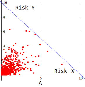
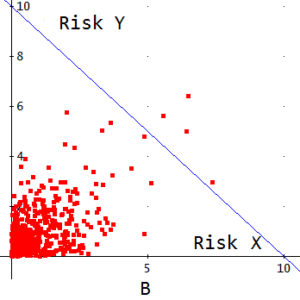
Risk X and risk Y have been simulated from the same distribution function and therefore have the same mean, variance, etc. However, both graphs A and B, differ in something very
important: In A there has not been any result where the sum of the amount of risk X plus the amount of Y exceeds 10 units, while in B there are some experiences that do exceed this threshold (represented in A and B by the straight diagonally descending line). Is this difference due to the fact that the correlation coefficient is greater in B than in A? No. In both cases the coefficient is 0.5. The greater severity of the risks (X, Y) in graph B stems from the different way in which these risks depend on each other, severity that is not reflected by the correlation coefficient.
This example leads us to the conclusion that any bivariate (and, in general, multivariate) distribution function involves two aspects defining the statistical behavior of these random variables:
- The marginal distribution of each one, that is, how it behaves statistically when observed in isolation from the other variable, and
- The joint behavior of both variables (i.e., the dependence structure). The copula is the function (in our example, function of two variables) that specifically regulates such joint behavior; therefore, the copula does not tell us anything about the marginal behavior of those variates.
To obtain the copula from a distribution function, we must “extract” the marginal distributions from it. What remains after this operation is the copula. If we have a distribution function of two variables F(x,y) with marginal distribution functions u=g(x), v=h(y), we know that these functions g and h determine the function F(x,y) so that in order to “isolate” or leave the copula function alone, we must “undo” the effect that g and h exert on F(x,y). This can be done in two steps:
First, we obtain the inverse functions g-1 and h-1. This is done by solving u=g(x) and v=h(y) for x and y respectively. We thus obtain x= g-1(u), y= h-1(v). We note that u and v represent the probability corresponding to each value of x and y according to the marginal distribution function g and h. So, the range of u and v is the interval (0 -1).
Next, we insert the expressions x = g-1(u) and y= h-1(v), into F(x,y). It thus follows that F(x, y) = F[g-1(u), h-1(v)] is, in short, a function that depends on u and v that is typically designated by C(u,v), and is called a copula.
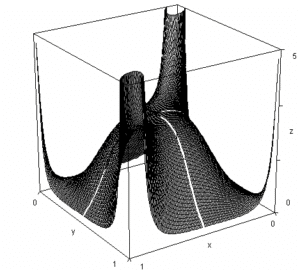
The copula is, therefore, “what remains” of a distribution function once the marginal behavior of the random variables is eliminated. Therefore it is the element that regulates and determines the dependence structure between those variables. The copula is a function defined for values between 0 and 1 of its independent variables u, v. Actually, it is the joint distribution function of these uniform variables (0,1) designated by u, v. The following graph shows the density function of the copula corresponding to a t-distribution with 4 degrees of freedom and a correlation coefficient of 0.6.

We have obtained the copula from a distribution function. In fact, it is also possible to follow the opposite route: To arrive at the distribution function by “connecting” the marginal distribution functions to the copula. That is, we would symbolically have:
Copula + marginal distributions = Joint distribution function
And also,
Joint distribution function – Marginal distributions = Copula
The possibility of combining a particular copula model with different distribution functions and, likewise, a certain set of copulas with different copula models, opens up a variety of different models for describing the joint statistical behavior of two or more random variables (i.e. of joint distribution models).
We have already seen how a copula can be obtained from a known multinomial distribution (Gauss, t-distribution). However, different copula models can also be obtained if we build functions that meet the essential requirements for the result to be considered a copula. Thus, in addition to the aforementioned Gauss and Student copulas, there are many others such as Clayton, Gumbel, Frank, etc., so that the professional has a remarkable variety of options for modeling the phenomenon of interest.
What is, then, the use of copulas? Wherever there is a diversity of risks that may be dependent on each other, there will be scope for attempting to apply copulas. Regulations of financial institutions (banks and insurance companies) tend to include a plurality of risks that affect them in their solvency systems. Our interest will be not only on how these risks are distributed individually or separately (marginal distribution) but also on the way in which they depend on one another. It may be the case that, under normal conditions, there is no dependency between them, but when a crisis occurs, things get worse in all of them. In this situation, the correlation coefficient is not a suitable instrument, while the application of copula theory may in fact provide a satisfactory result. In the European Union regulations on insurance company solvency (Solvency II), the coefficient of correlation is in some cases increased so as to allow for the insufficiency of this coefficient. Despite the advantage of its simplicity, this solution seems too crude to us to be satisfactory. Thus, in such cases it is advisable to consider the application of copula theory, that offers models flexible enough to adapt to a wide variety of phenomena.
The interested reader may use my work entitled Teoría de Cópulas. Introducción y Aplicaciones a Solvencia II (Theory of Copulas. Introduction and Applications to Solvency II, only available in Spanish) (Fundación Mapfre) as an introduction to this topic, and subsequently continue with the study of the extensive literature available, proof of the great interest that it deserves among scholars and professionals of these issues.


